Joint categorical distribution diagnostic across groups

Runs a descriptive cross-group diagnostic for categorical data: marginal comparisons per variable, plus modality-level omnibus and edge-wise association-structure comparisons. Intended as the user-facing entry point for cross-group diagnostics in meta-analysis, multi-site studies, and repeated cross-sectional surveys.

Usage

joint_balance(
  data,
  group,
  variables = NULL,
  n_perm = 500L,
  n_perm_edge = NULL,
  alpha = 0.05,
  strata = NULL,
  run_edgewise = TRUE,
  seed = NULL,
  verbose = TRUE
)

# S3 method for class 'jointbalance'
print(x, ...)

# S3 method for class 'jointbalance'
summary(object, ...)

Arguments

data: A data frame of categorical variables plus a grouping column.
group: Character. Name of the grouping column in data. Must be categorical with at least 2 levels.
variables: Optional character vector. Names of columns to include in the joint analysis. Default NULL uses all columns in data other than group.
n_perm: Integer. Permutations for the omnibus test, passed to test_modality_graph_equality. Default 500L.
n_perm_edge: Integer. Permutations for the edge-wise post-hoc test. Default equal to n_perm.
alpha: Numeric. Significance level reported for all three testing families. Default 0.05.
strata: Optional stratification vector passed through to the omnibus and edge-wise tests. Length must equal nrow(data).
run_edgewise: Logical. If TRUE (default), runs test_modality_edge_differences for each pair whose omnibus test rejects at alpha. Set to FALSE to skip the post-hoc step (faster, useful when you only want the balance summary).
seed: Optional integer seed.
verbose: Logical. If TRUE (default), prints progress.
x: A jointbalance object.
...: Ignored.
object: A jointbalance object.

Value

An object of class jointbalance with components:

group: Name of the grouping variable.
group_levels: Character vector of group levels.
variables: Character vector of analysed variables.
marginal: Data frame, one row per variable: variable, chisq, df, p_value, p_adjusted, cramers_v. Adjustment is BH across variables.
pairwise_omnibus: Data frame, one row per group pair: group_x, group_y, n_x, n_y, statistic, observed, p_value, p_bonferroni. Adjustment is Bonferroni across pairs.
pairwise_edgewise: Named list of catmodedgetest objects, one per pair that rejected the omnibus (empty if none did or run_edgewise = FALSE). Names are "\{group_x\}_vs_\{group_y\}".
modality_graphs: Named list of catmodgraph objects, one per group level.
alpha: The alpha used.
call: The matched call.

Details

What this function reports, in plain terms.

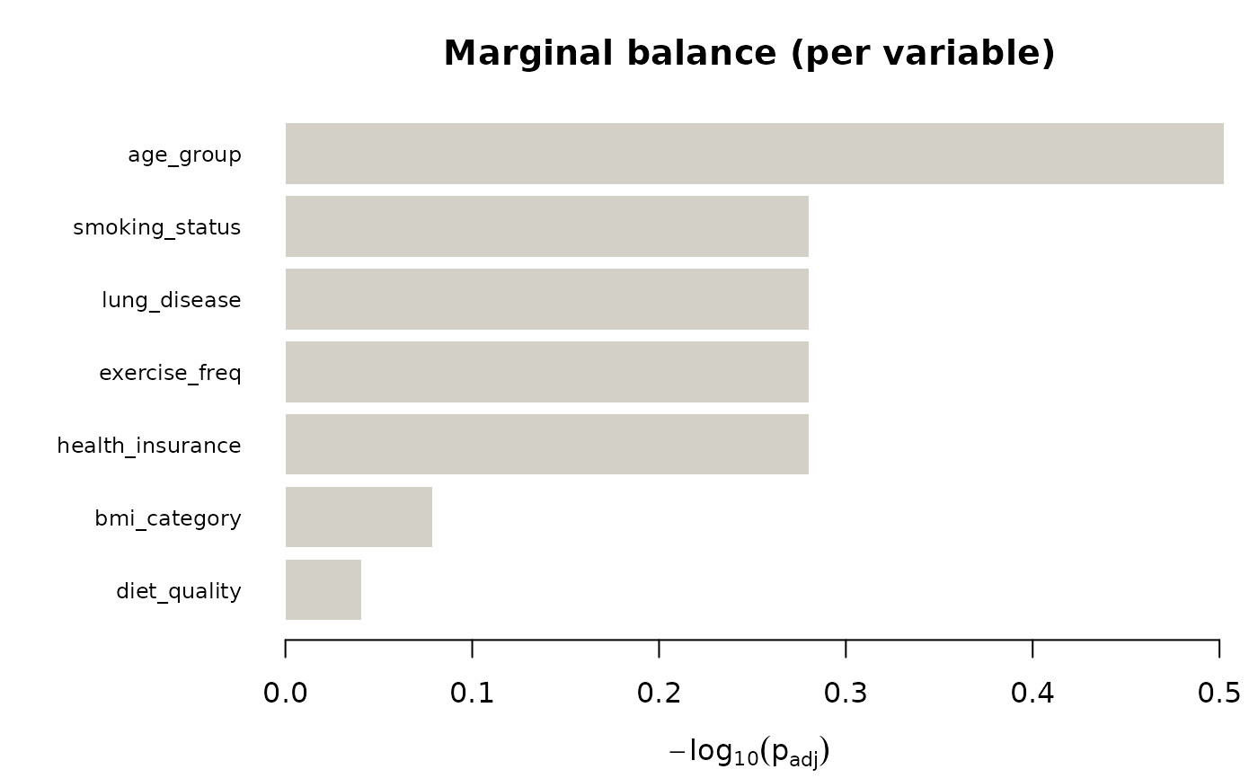
Marginal balance (the classical "Table 1" check): is each variable distributed the same across groups, one variable at a time?
Joint balance (the modality network test): is the full joint categorical structure the same across groups?
Where the joint structure differs (the edge-wise post-hoc): which modality-pair associations account for any joint disagreement?

Marginal similarity is not sufficient to establish similarity of joint categorical association structure. Two groups with identical marginals can still differ in joint structure — for example, if variable A and variable B are positively associated in group 1 and negatively associated in group 2, both groups will show the same one-way marginals for A and for B, but the joint distribution will differ. This is exactly the scenario the modality-layer test is designed to catch, and it is the reason a joint-structure diagnostic can reveal discrepancies that marginal-only Table 1 summaries may miss.

Interpretation. The diagnostic compares observed categorical distributions and modality-level association patterns across groups. It does not establish exchangeability, causal comparability, or absence of residual confounding. Results should be interpreted as evidence of distributional and associational discrepancies, not as proof that groups are or are not analytically interchangeable.

Testing families and multiplicity. Three separate multiple-testing corrections are applied:

Marginal tests: Benjamini-Hochberg FDR across the \(p\) variables. Exploratory; the marginal panel of the plot is meant to triage, not to make definitive claims.
Omnibus tests across group pairs: Bonferroni across the \(\binom{k}{2}\) pairs. Conservative by design, because these pairwise tests are logically nested (rejecting "wave 1 vs wave 2" and "wave 1 vs wave 3" both implicate wave 1).
Edge-wise post-hoc within each pair: Benjamini-Hochberg across edges, as done by test_modality_edge_differences. This is a conditional family, valid under the closed-testing principle only if the omnibus rejected.

These are three separate testing families, not one big correction. The print method makes this distinction explicit.

When not to use this. joint_balance() is a descriptive diagnostic for fully categorical data. It is not a causal adjustment tool and does not replace propensity-score or entropy-balancing workflows. For continuous covariates use the cobalt or tableone packages; this function silently coerces numeric columns to factors if they appear in variables, which is almost never what you want.

Functions

print(jointbalance): Print a concise diagnostic summary.
summary(jointbalance): Return the key diagnostic tables.

References

The marginal/joint distinction is a long-standing one in log-linear modelling; see Agresti (2013), Categorical Data Analysis (3rd ed.), Wiley, chapter 9, for homogeneity-of- association tests built from three-way log-linear models. The permutation approach used here is an alternative that avoids the large-sample assumptions of the likelihood-ratio test.

Examples

# \donttest{
data(survey_health)
jb <- joint_balance(
  survey_health, group = "sex",
  n_perm = 200, n_perm_edge = 200, seed = 1, verbose = FALSE
)
jb
#> jointbalance diagnostic
#>   Group variable : sex 
#>   Levels         : female, male 
#>   Variables      : 7 ( age_group, smoking_status, lung_disease, exercise_freq, bmi_category , ... )
#>   Alpha          : 0.05 
#> 
#> Marginal tests (BH-adjusted across variables):
#>   Variables rejecting at alpha : 0 / 7 
#> 
#> Pairwise omnibus tests (Bonferroni across group pairs):
#>   Pairs rejecting at alpha     : 0 / 1 
#> 
#> Three separate testing families; see ?joint_balance for details.
summary(jb)
#> $marginal_table
#>           variable     chisq df    p_value  cramers_v p_adjusted
#> 1        age_group 6.2042760  2 0.04495299 0.10718862  0.3146709
#> 2   smoking_status 2.6730409  2 0.26275837 0.07022684  0.5246600
#> 3     lung_disease 0.7878298  1 0.37475715 0.03812559  0.5246600
#> 4    exercise_freq 2.7482263  2 0.25306393 0.07120764  0.5246600
#> 5     bmi_category 1.3596640  3 0.71501635 0.04994794  0.8341857
#> 6     diet_quality 0.1868313  2 0.91081486 0.01860064  0.9108149
#> 7 health_insurance 0.9263115  1 0.33582322 0.04137899  0.5246600
#> 
#> $pairwise_omnibus_table
#>   group_x group_y n_x n_y statistic observed   p_value p_bonferroni
#> 1  female    male 206 195 frobenius 1.911981 0.1492537    0.1492537
#> 
#> $n_edgewise_pairs
#> [1] 0
#> 
#> $group
#> [1] "sex"
#> 
#> $group_levels
#> [1] "female" "male"  
#> 
#> $alpha
#> [1] 0.05
#> 
plot(jb)
#> No pair rejected the omnibus at alpha = 0.05; falling back to layout = 'marginal_only'.

# }