Plot a modality graph

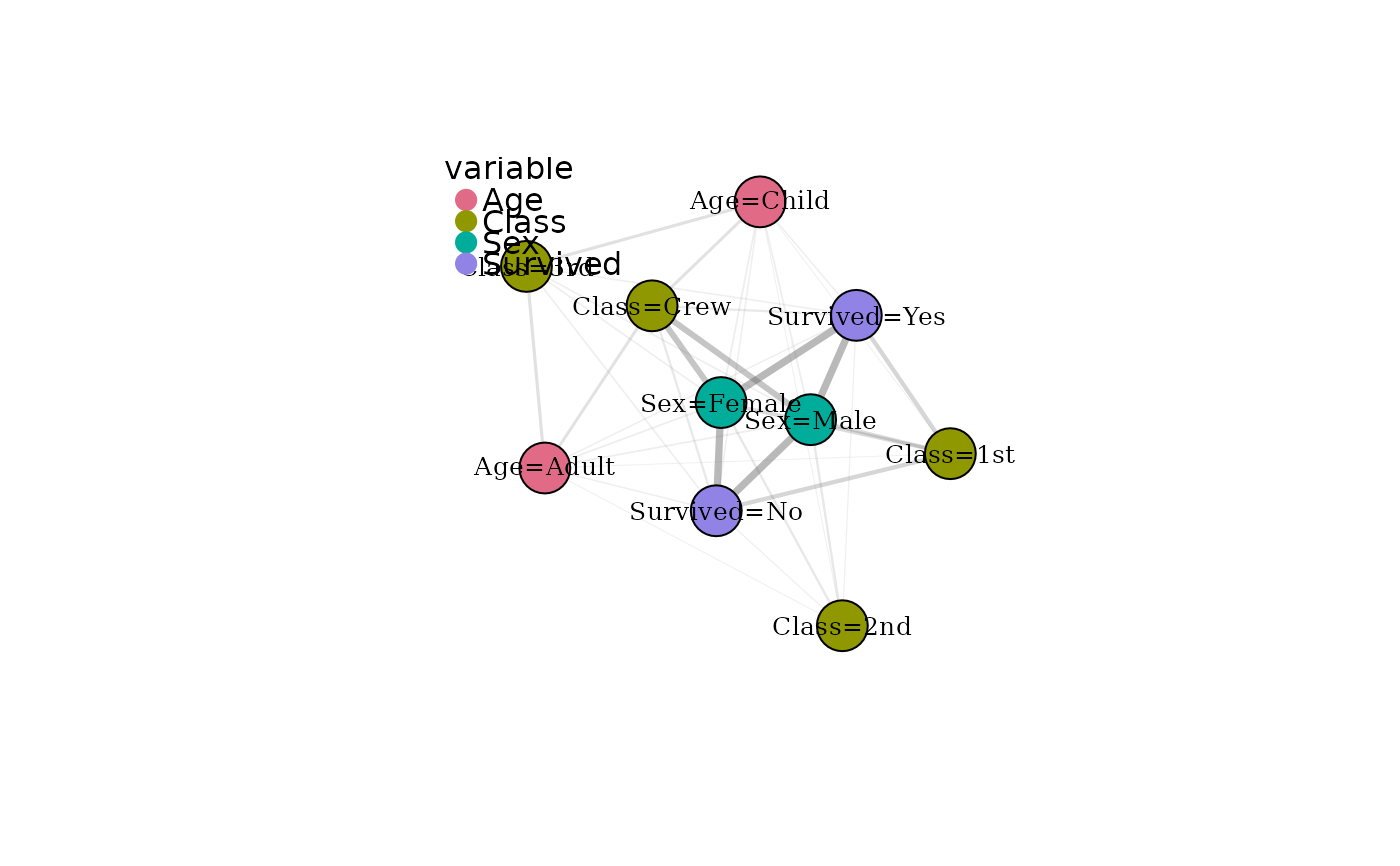
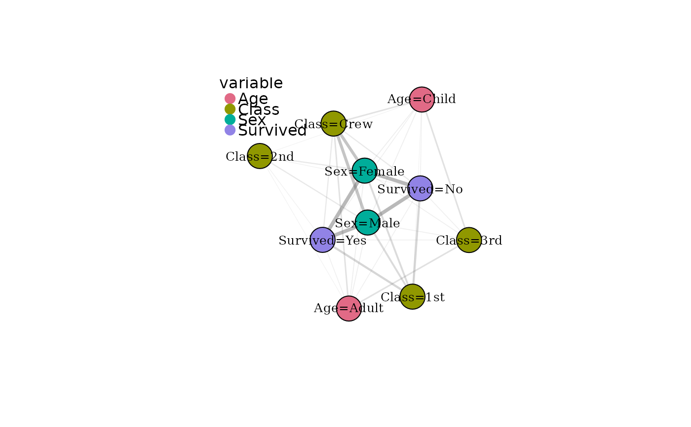
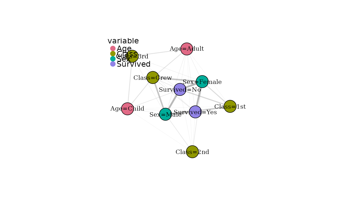
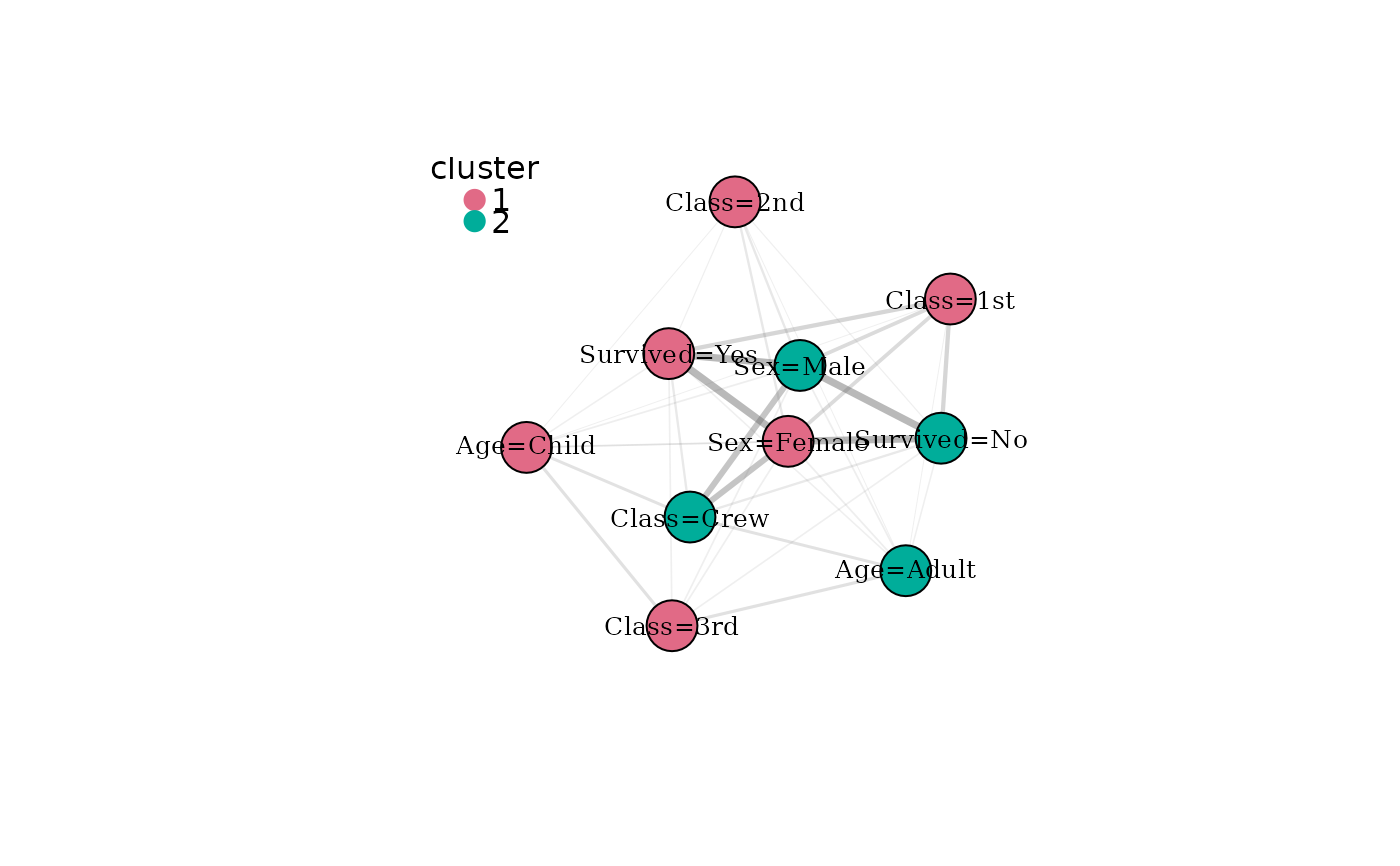
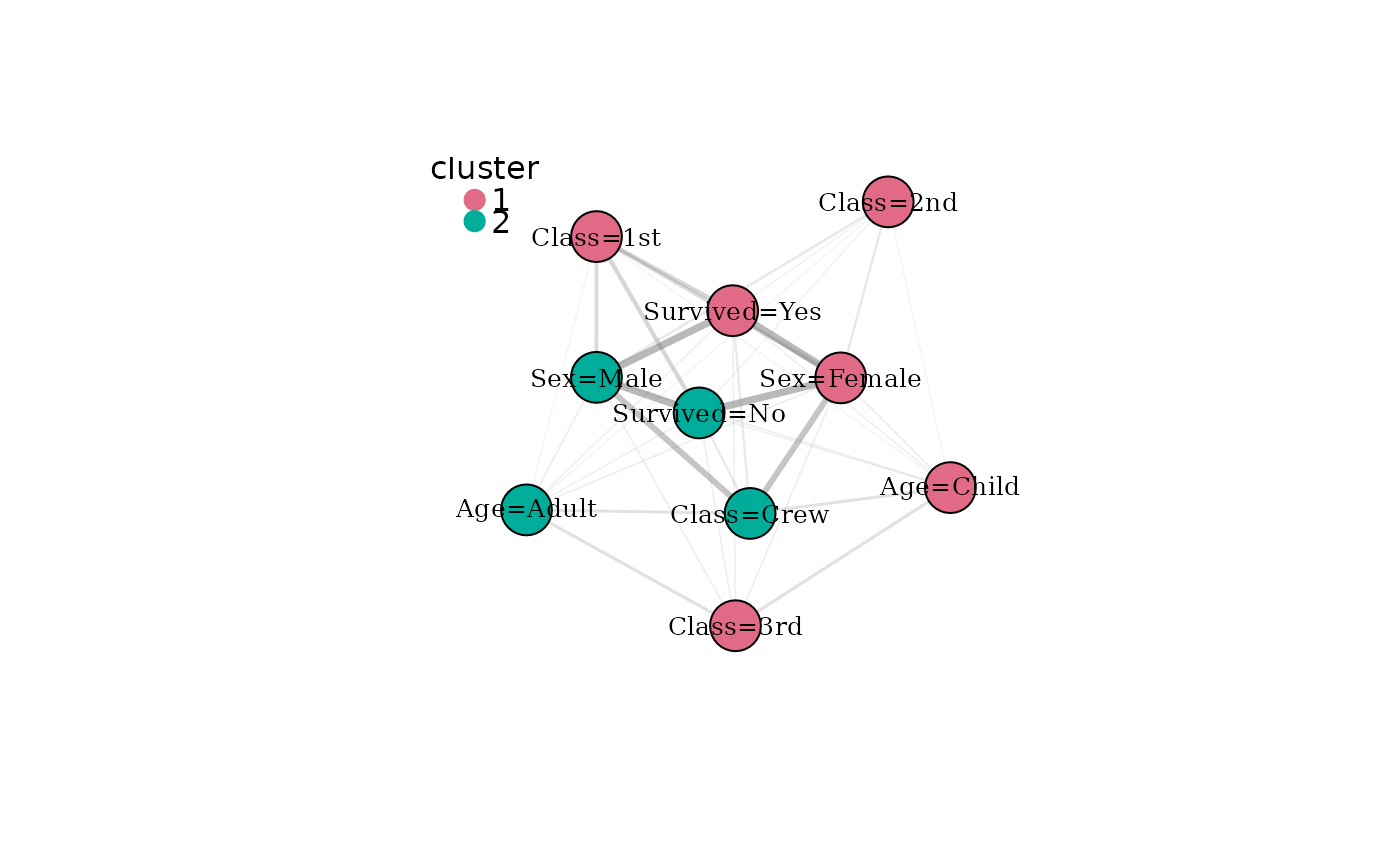
Visualises a catmodgraph object. Nodes represent modalities and edges represent cross-variable modality associations. By default, node colours indicate the originating variable. If modality communities have been detected, colours can instead reflect community membership.

Usage

# S3 method for class 'catmodgraph'
plot(
  x,
  color_by = c("variable", "cluster"),
  signed = FALSE,
  show_labels = TRUE,
  layout = c("fr", "kk"),
  vertex_size = 24,
  edge_scale = 8,
  remove_isolates = TRUE,
  ...
)

Arguments

x

A catmodgraph object.

color_by

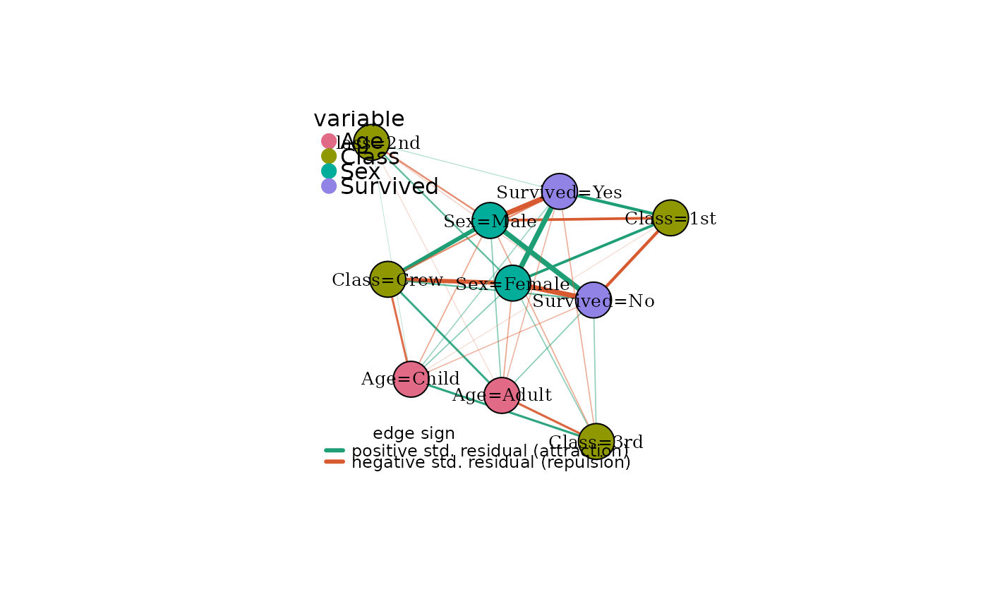
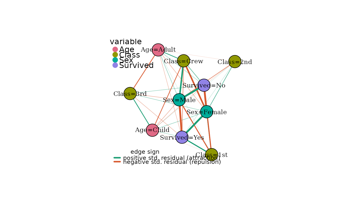
Character. One of "variable" (default) or "cluster".

signed

Logical. If TRUE, edge colour encodes the sign of the stored standardised Pearson residual: green for positive (attraction), red for negative (repulsion). Default is FALSE, which uses a uniform grey edge colour. Requires the std_resid edge attribute (present by default in graphs built with build_modality_graph).

show_labels

Logical. If TRUE, node labels are drawn. Default is TRUE.

layout

Character. Graph layout passed to igraph::layout_with_fr() or igraph::layout_with_kk(). One of "fr" (default) or "kk".

vertex_size

Numeric. Node size. Default is 24.

edge_scale

Numeric. Multiplicative factor applied to edge widths. Default is 8.

remove_isolates

Logical. If TRUE (default), vertices with degree 0 are hidden from the plot. Isolated modalities typically arise after pruning and carry no community structure information, so removing them improves interpretability. Set to FALSE to see every vertex in the graph. Does not modify the input object.

...

Further arguments passed to plot.igraph().

Value

Invisibly returns the input object.

Details

When signed = TRUE, edges are coloured by the sign of the stored standardised Pearson residual (std_resid edge attribute): green for positive (modalities co-occurring more than expected under independence) and red for negative (co-occurring less than expected). Edge alpha transparency then scales with |std_resid|.

Examples

df <- expand_table(Titanic)
mg <- build_modality_graph(df)
mg <- cluster_modalities(mg)

# Base plotting
plot(mg)


# Colour nodes by detected modality community
plot(mg, color_by = "cluster")


# Signed edges: green = attraction, red = repulsion
plot(mg, signed = TRUE)


df <- expand_table(Titanic)
mg <- build_modality_graph(df)
mg <- cluster_modalities(mg)

# Base plotting
plot(mg)


# Colour nodes by detected modality community
plot(mg, color_by = "cluster")


# Signed edges: green = attraction, red = repulsion
plot(mg, signed = TRUE)


# Show isolated vertices (not hidden by default)
plot(mg, remove_isolates = FALSE)